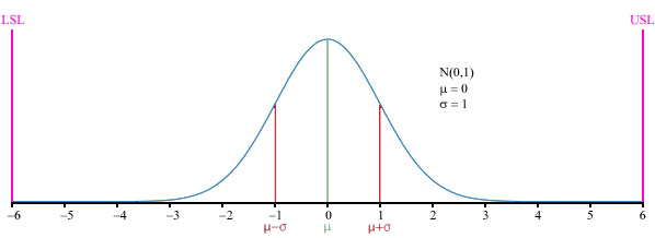
Graph of the normal distribution, which underlies the statistical assumptions of the Six Sigma model. The Greek letter σ (segma) marks the distance on the horizontal axis between the mean, µ, and the curve's inflection point, in this case σ=1. The distance is equally distributed horizontally to both sides of the mean µ as: [µ - σ/2, µ + σ/2]. The greater this distance, the greater is the spread of values encountered. For the curve shown above, µ = 0 and σ = 1. The upper and lower specification limits (USL, LSL) are at a distance of 6σ from the mean. Because of the properties of the normal distribution, values lying that far away from the mean are extremely unlikely. Even if the mean were to move right or left by 1.5σ at some point in the future (1.5 sigma shift), there is still a good safety cushion. This is why Six Sigma aims to have processes where the mean is at least 6σ away from the nearest specification limit.
The term "six sigma process" comes from the notion that if one has six standard deviations between the process mean and the nearest specification limit, as shown in the graph, practically no items will fail to meet specifications. This is based on the calculation method employed in process capability studies.
Capability studies measure the number of standard deviations between the process mean and the nearest specification limit in sigma units. As process standard deviation goes up, or the mean of the process moves away from the center of the tolerance, fewer standard deviations will fit between the mean and the nearest specification limit, decreasing the sigma number and increasing the likelihood of items outside specification.

Role of the 1.5 sigma shift
Experience has shown that in the long term, processes usually do not perform as well as they do in the short.   As a result, the number of sigmas that will fit between the process mean and the nearest specification limit may well drop over time, compared to an initial short-term study. To account for this real-life increase in process variation over time, an empirically-based 1.5 sigma shift is introduced into the calculation. According to this idea, a process that fits six sigmas between the process mean and the nearest specification limit in a short-term study will in the long term only fit 4.5 sigmas – either because the process mean will move over time, or because the long-term standard deviation of the process will be greater than that observed in the short term, or both.
Hence the widely accepted definition of a six sigma process as one that produces 3.4 defective parts per million opportunities (DPMO). This is based on the fact that a process that is normally distributedwill have 3.4 parts per million beyond a point that is 4.5 standard deviations above or below the mean (one-sided capability study). So the 3.4 DPMO of a "Six Sigma" process in fact corresponds to 4.5 sigmas, namely 6 sigmas minus the 1.5 sigma shift introduced to account for long-term variation. . The theory behind this is that over a longer period of time there are likely to be special causes that do not accurately reflect the behaviour of the process/business. These special causes are likely to have an effect of deteriorating process performance This is designed to prevent underestimation of the defect levels likely to be encountered in real-life operation.

Sigma levels

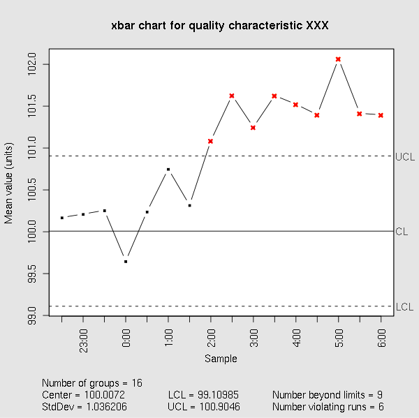
A control chart depicting a process that experienced a 1.5 sigma drift in the process mean toward the upper specification limit starting at midnight. Control charts are used to maintain 6 sigma quality by signaling when quality professionals should investigate a process to find and eliminate special-cause variation.

The table below gives long-term DPMO values corresponding to various short-term sigma levels.
Note that these figures assume that the process mean will shift by 1.5 sigma toward the side with the critical specification limit. In other words, they assume that after the initial study determining the short-term sigma level, the long-term Cpk value will turn out to be 0.5 less than the short-term Cpk value. So, for example, the DPMO figure given for 1 sigma assumes that the long-term process mean will be 0.5 sigma beyond the specification limit (Cpk = –0.17), rather than 1 sigma within it, as it was in the short-term study (Cpk = 0.33). Note that the defect percentages only indicate defects exceeding the specification limit to which the process mean is nearest. Defects beyond the far specification limit are not included in the percentages.